Script 1 - Estimators

Author

Alice Giampino

mu.true <- 27.3
sigma2.true <- 1
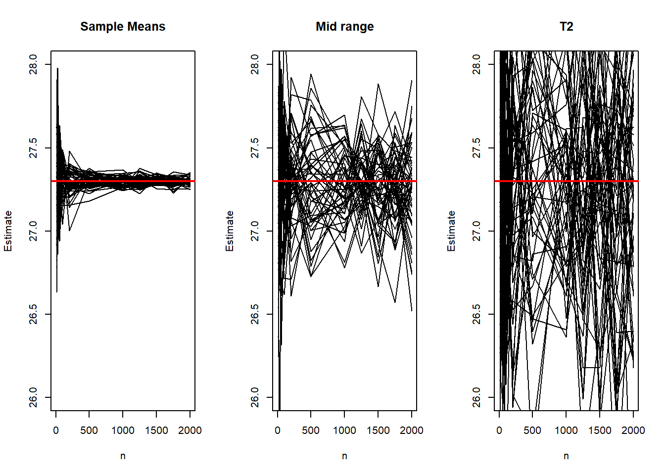
sample_sizes <- c(10, 25, 50, 100, 200,
                  500, 1000,1250, 1500, 1750, 2000)

B <- length(sample_sizes)
N_samples <- 50

mean_est <- matrix(NA, nrow=B, ncol=N_samples)
T_range <- matrix(NA, nrow=B, ncol=N_samples)
T_2 <- matrix(NA, nrow=B, ncol=N_samples)


set.seed(6)
for(i in 1:B){
  for(j in 1:N_samples){
    n <- sample_sizes[i]
    
    y <- rnorm(n, mean=mu.true, sd=sqrt(sigma2.true))
    mean_est[i,j] <- mean(y)
    T_range[i,j] <- (min(y) + max(y))/2
    T_2[i,j] <- (y[1] + y[n])/2
  }
}

par(mfrow=c(1,3))
plot(sample_sizes, mean_est[,1], type="l", ylim=c(26,28), 
     main = "Sample Means", ylab = "Estimate", xlab = "n")

for(i in 2:N_samples){
  points(sample_sizes, mean_est[,i], type="l")
}
abline(h=mu.true, col="red", lwd=2)

################################################
plot(sample_sizes, T_range[,1], type="l", ylim=c(26,28), 
     main = "Mid range", ylab = "Estimate", xlab = "n")

for(i in 2:N_samples){
  points(sample_sizes, T_range[,i], type="l")
}
abline(h=mu.true, col="red", lwd=2)

################################################
plot(sample_sizes, T_2[,1], type="l", ylim=c(26,28), 
     main = "T2", ylab = "Estimate", xlab = "n")

for(i in 2:N_samples){
  points(sample_sizes, T_2[,i], type="l")
}
abline(h=mu.true, col="red",lwd=2)

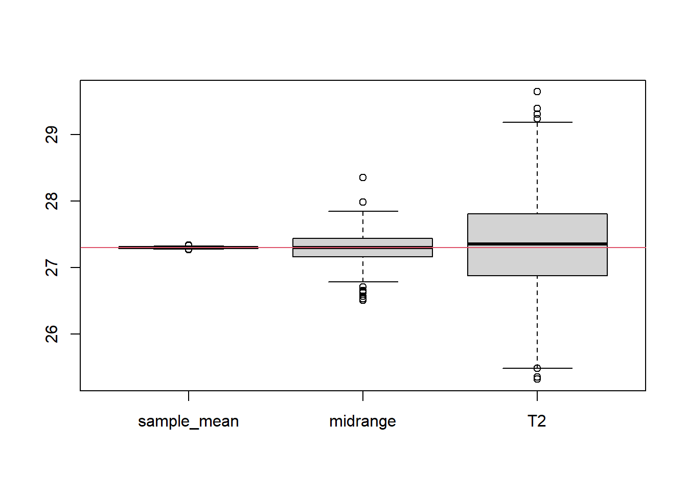
par(mfrow=c(1,1))




# Let's replicate the estimation procedure for n=10000

B <- 1000
mean_est <- numeric(B)
T_range <- numeric(B)
T_2 <- numeric(B)
for(i in 1:B){

  y <- rnorm(10000, mean=mu.true, sd=sqrt(sigma2.true))
  mean_est[i] <- mean(y)
  T_range[i] <- (min(y) + max(y))/2
  T_2[i] <- (y[1] + y[10000])/2
}

boxplot(cbind(sample_mean=mean_est,
              midrange=T_range,
              T2=T_2))
abline(h=mu.true, col=2)

##############################################
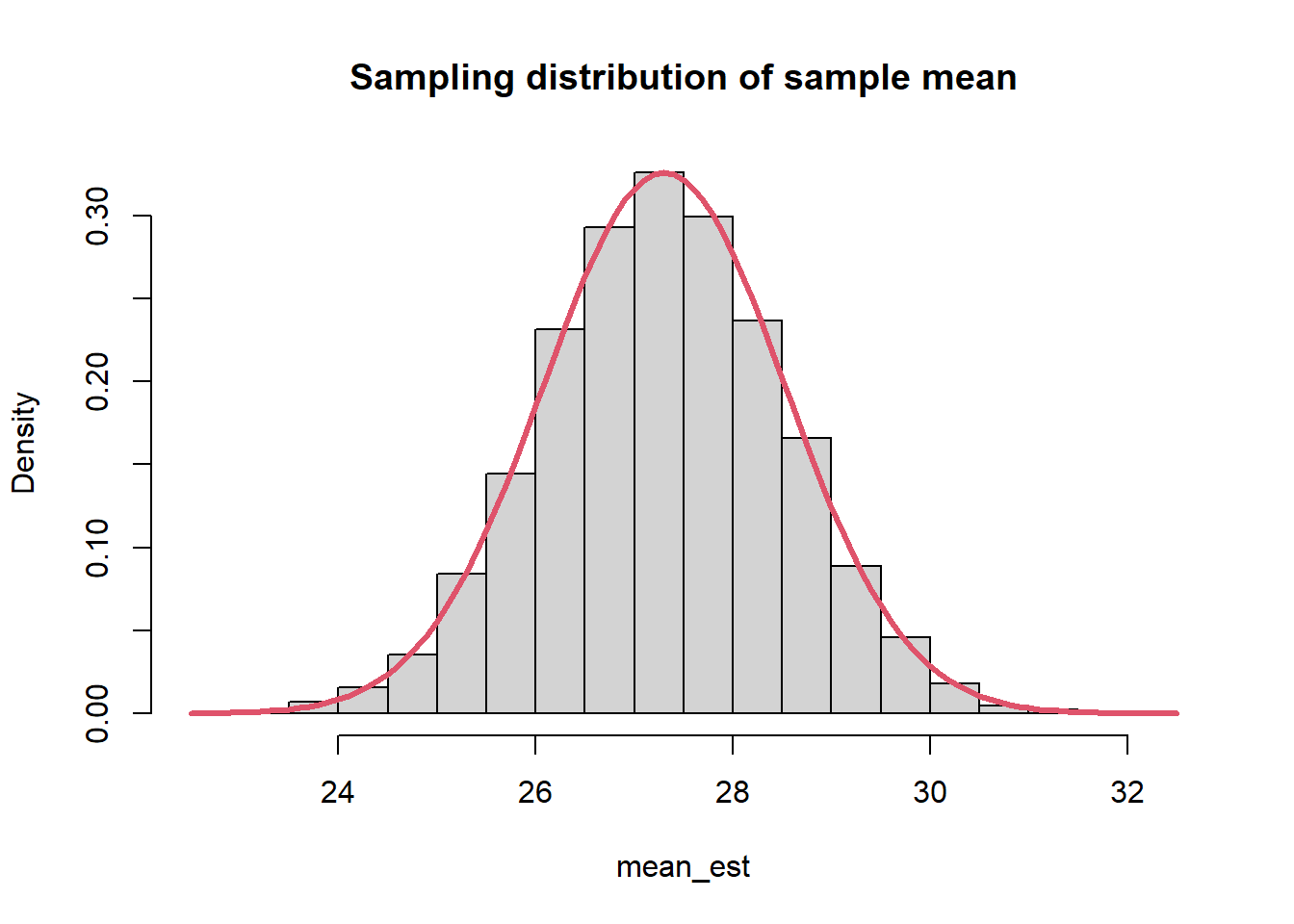
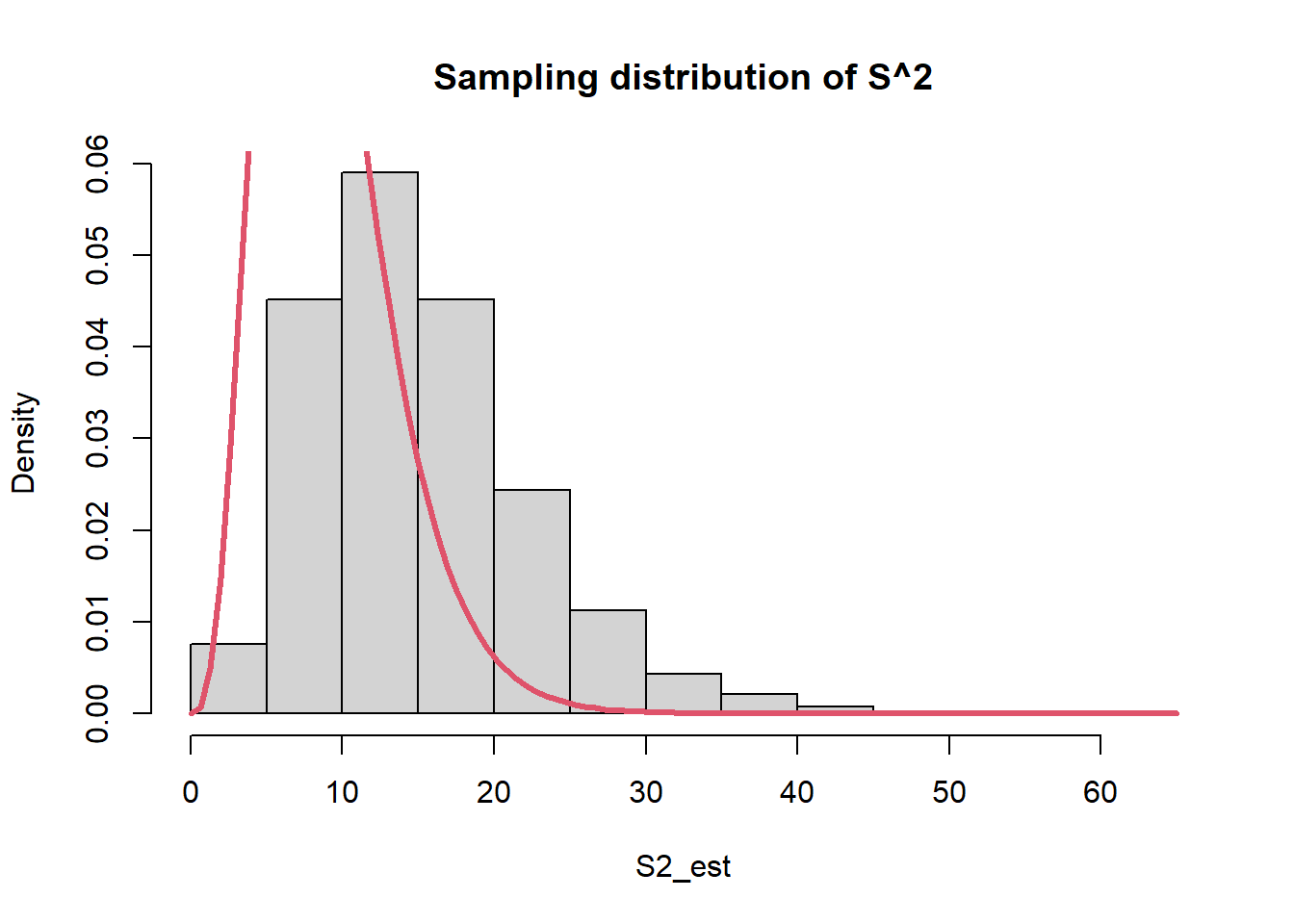
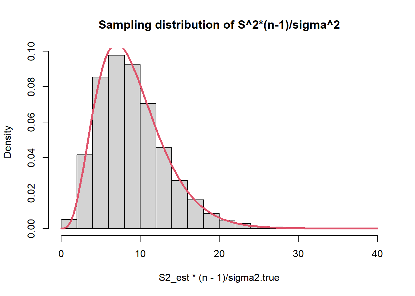
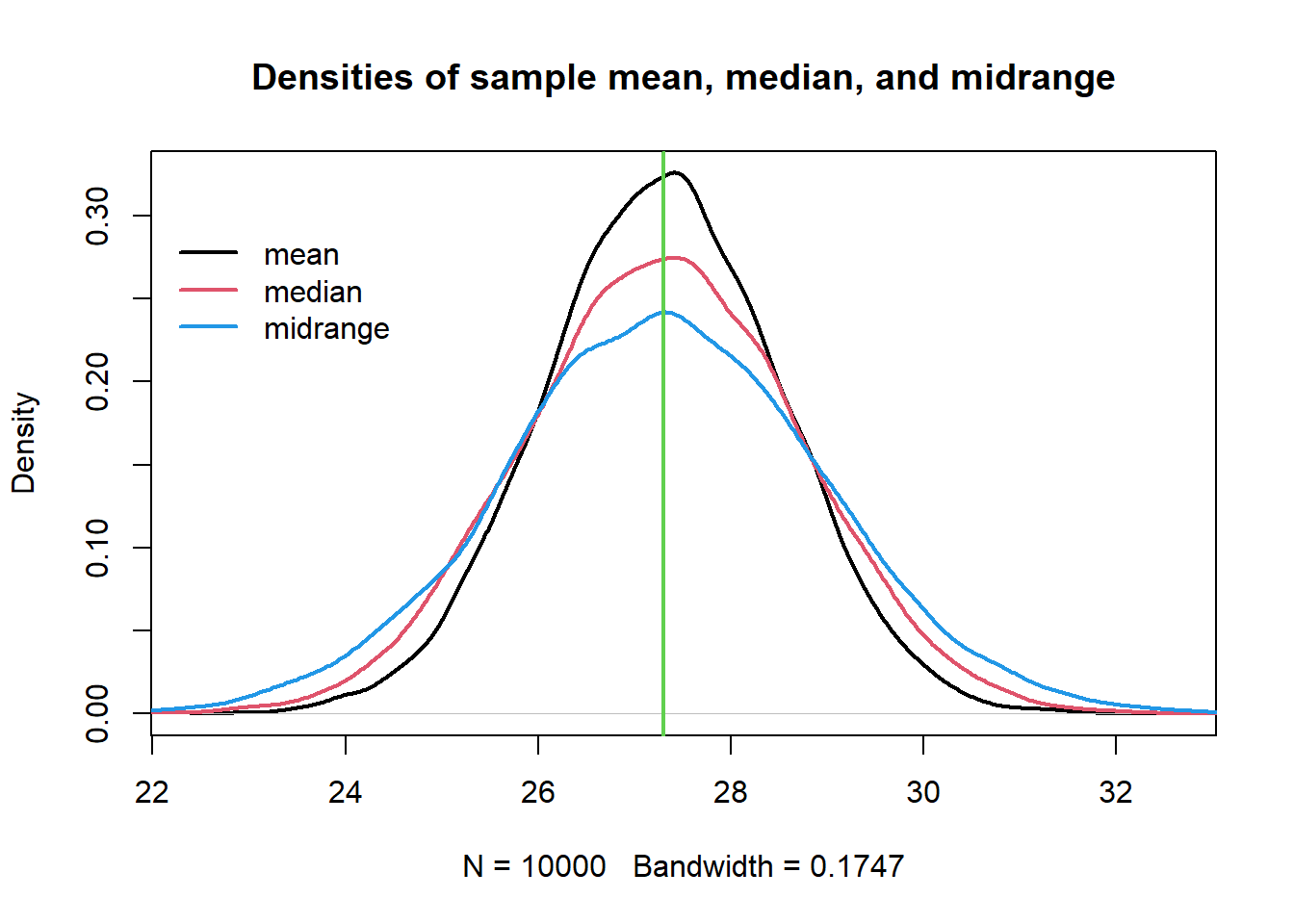
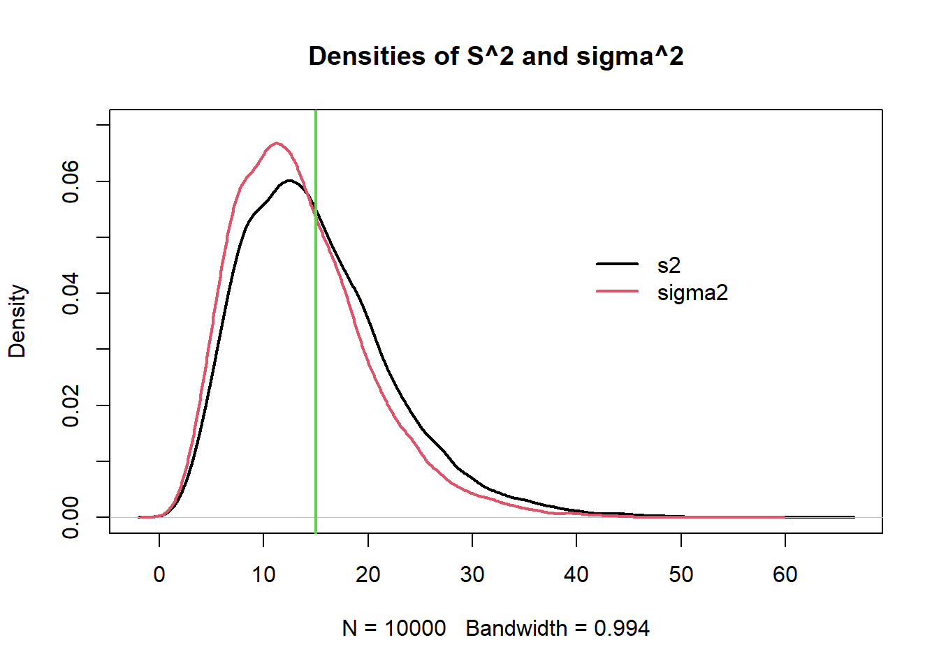
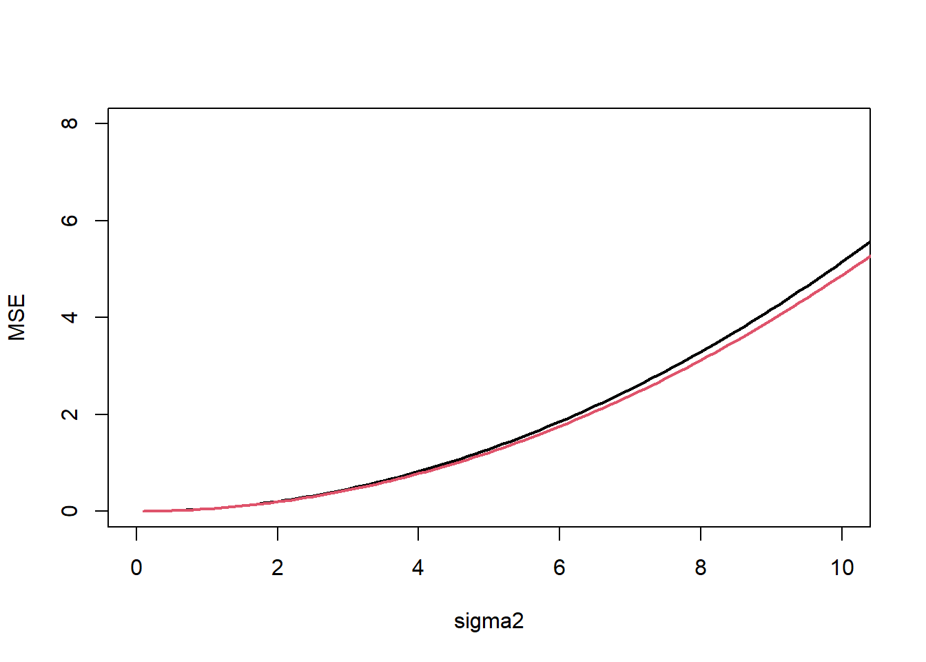
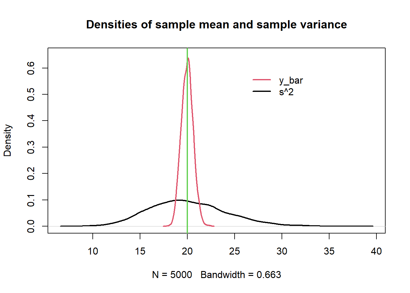
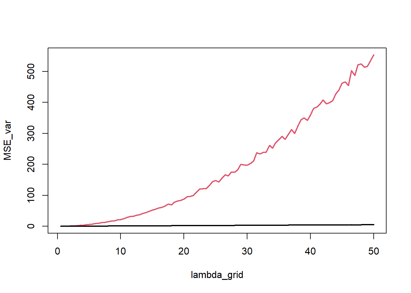
######## 1.2 - Comparing estimators: #########
##############################################

mu.true <- 27.3
sigma2.true <- 15
n <- 10


# Sampling distributions:
B <- 10000
mean_est <- numeric(B)
median_est <- numeric(B)
T_range <- numeric(B)

S2_est <- numeric(B)
sigma2_est <- numeric(B)

set.seed(6)
for(b in 1:B){
  y <- rnorm(n, mean=mu.true, sd=sqrt(sigma2.true))
  mean_est[b] <- mean(y)
  median_est[b] <- median(y)
  T_range[b] <- (min(y) + max(y))/2

  S2_est[b] <- var(y)
  sigma2_est[b] <- var(y)*(n-1)/n
}

hist(mean_est, prob=T, main="Sampling distribution of sample mean")
curve(dnorm(x, mu.true, sd=sqrt(sigma2.true/n)), col=2, lwd=3,add=T)

hist(S2_est, prob=T, main="Sampling distribution of S^2")
curve(dchisq(x, n-1), col=2, add=T, lwd=3)

hist(S2_est*(n-1)/sigma2.true, prob=T, main="Sampling distribution of S^2*(n-1)/sigma^2")
curve(dchisq(x, n-1), col=2, add=T, lwd=3)

# Expected values (approximated):

mean(mean_est)

[1] 27.29257

mean(median_est)

[1] 27.28862

mean(T_range)

[1] 27.29507

mean(S2_est)

[1] 15.06223

mean(sigma2_est)

[1] 13.55601

# Biases (approximated):

mean(mean_est) - mu.true

[1] -0.007429892

mean(median_est) - mu.true

[1] -0.01138043

mean(T_range) - mu.true

[1] -0.004933008

mean(S2_est) - sigma2.true

[1] 0.06223293

mean(sigma2_est) - sigma2.true

[1] -1.44399

# MSEs (approximated):

mean((mean_est - mu.true)^2)

[1] 1.500696

mean((median_est - mu.true)^2)

[1] 2.061422

mean((T_range - mu.true)^2)

[1] 2.833997

mean((S2_est - sigma2.true)^2)

[1] 52.32536

mean((sigma2_est- sigma2.true)^2)

[1] 44.46551

# Bias-variance trade-off (it holds for B >> 0, it is approximated):
mean((mean_est - mu.true)^2)

[1] 1.500696

(mean(mean_est) - mu.true)^2 + var(mean_est)*(B-1)/B

[1] 1.500696

# Other measures:
# MAEs (approximated):

mean(abs(mean_est - mu.true))

[1] 0.9773448

mean(abs(median_est - mu.true))

[1] 1.146815

mean(abs(T_range - mu.true))

[1] 1.332213

mean(abs(S2_est - sigma2.true))

[1] 5.626325

mean(abs(sigma2_est- sigma2.true))

[1] 5.372079

# ARB Absolute relative bias (approximated):

mean(abs(mean_est - mu.true)/mu.true)

[1] 0.03580018

mean(abs(median_est - mu.true)/mu.true)

[1] 0.04200787

mean(abs(T_range - mu.true)/mu.true)

[1] 0.048799

mean(abs(S2_est - sigma2.true)/sigma2.true)

[1] 0.3750883

mean(abs(sigma2_est- sigma2.true)/sigma2.true)

[1] 0.3581386

# Sampling Distributions:
plot(density(mean_est), main="Densities of sample mean, median, and midrange", lwd=2)
lines(density(median_est),  col=2, lwd=2)
lines(density(T_range),  col=4, lwd=2)
abline(v=mu.true, col=3, lwd=2)
legend(22,.3, legend=c("mean", "median", "midrange"), col=c(1:2,4), lty=1, lwd=2, bty = "n")

plot(density(S2_est), main="Densities of S^2 and sigma^2", ylim=c(0,0.07), lwd=2)
lines(density(sigma2_est),  col=2, lwd=2)
abline(v=sigma2.true, col=3, lwd=2)
legend(40,.05, legend=c("s2", "sigma2"), col=1:2, lty=1, bty = "n", lwd=2)

#####################################################
##### 1.3 - Comparing estimators for variance: ######
#####################################################

# This function returns the MSE of S^2 and sigma2_hat
# approximated with B replicates

mse_normal_sigma2 <- function(mu, sigma2, n, B){

  est_s2 <- numeric(B)
  est_sigma2 <- numeric(B)

  set.seed(42)
  for(b in 1:B){
    y <- rnorm(n, mu, sqrt(sigma2))

    est_s2[b] <- var(y)
    est_sigma2[b] <- ((n-1)/n)*var(y)

  }

  mse_s2 <- mean((est_s2-sigma2)^2)
  mse_sigma2 <- mean((est_sigma2-sigma2)^2)

  return(c(mse_s2, mse_sigma2))
}

mse_normal_sigma2(mu=10, sigma2=15, n=10, B=50)

[1] 46.76627 41.98079

# Grid of values for (the true) sigma2
sigma2_vector <- seq(0.1, 50, by=0.1)
B <- 1000

mse_s2 <- numeric(length(sigma2_vector))
mse_sigma2 <- numeric(length(sigma2_vector))

for(s in 1:length(sigma2_vector)){
  mse <- mse_normal_sigma2(10, sigma2_vector[s], 40, B)

  mse_s2[s] <- mse[1]
  mse_sigma2[s] <- mse[2]
}

plot(sigma2_vector, mse_s2, pch=20,
     type="l", ylab="MSE", xlab="sigma2", lwd=2, xlim=c(0,10),
     ylim=c(0,8))
points(sigma2_vector, mse_sigma2, pch=20, type="l", col=2, lwd=2)

legend(0,150, legend=c("S2", "sigma2_hat"), col=c(1,2), lty=1, bty="n", lwd=2)

################################################
##### 1.4 - Comparing estimators Poisson: ######
################################################

lambda <- 20
n <- 50
B <- 5000

est_mean <- numeric(B)
est_s2 <- numeric(B)

set.seed(369)
for(b in 1:B){
  y <- rpois(n, lambda)

  est_mean[b] <- mean(y)
  est_s2[b] <- var(y)
}

mse_mean <- mean((est_mean-lambda)^2); mse_mean

[1] 0.3946222

mse_s2 <- mean((est_s2-lambda)^2); mse_s2

[1] 16.37713

plot(density(est_s2), main="Densities of sample mean and sample variance",
     ylim=c(0,.65), lwd=2)
lines(density(est_mean),  col=2, lwd=2)
abline(v=lambda, col=3, lwd=2)
legend(26,.6, legend=c("y_bar", "s^2"), col=2:1, lty=1, bty = "n", lwd=2)

n <- 10
B <- 5000
lambda_grid <- seq(0.5, 50, by=.5)

MSE_mean <- numeric(length(lambda_grid))
MSE_var <- numeric(length(lambda_grid))

for(l in 1:length(lambda_grid)){
  
  stime_media <- numeric(B)
  stime_var <- numeric(B)
  
  for(b in 1:B){
    x <- rpois(n, lambda=lambda_grid[l])
    
    stime_media[b] <- mean(x)
    stime_var[b] <- var(x)
  }
  
  MSE_mean[l] <- mean((stime_media - lambda_grid[l])^2)
  MSE_var[l] <- mean((stime_var - lambda_grid[l])^2)
}

plot(lambda_grid, MSE_var, type="l", col=2, lwd=2)
points(lambda_grid, MSE_mean, type="l", lwd=2)