Script 6 - Linear Model

#Cherry tress data:
data(trees)
# help(trees)
n <- nrow(trees)

summary(trees)

     Girth           Height       Volume     
 Min.   : 8.30   Min.   :63   Min.   :10.20  
 1st Qu.:11.05   1st Qu.:72   1st Qu.:19.40  
 Median :12.90   Median :76   Median :24.20  
 Mean   :13.25   Mean   :76   Mean   :30.17  
 3rd Qu.:15.25   3rd Qu.:80   3rd Qu.:37.30  
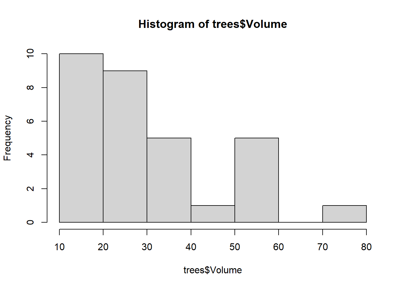
 Max.   :20.60   Max.   :87   Max.   :77.00  

colnames(trees)[1] <- "Diameter"

hist(trees$Volume)

hist(trees$Diameter)

hist(trees$Height)

plot(trees, pch=19)

cor(trees[,1:3])

          Diameter    Height    Volume
Diameter 1.0000000 0.5192801 0.9671194
Height   0.5192801 1.0000000 0.5982497
Volume   0.9671194 0.5982497 1.0000000

#################################
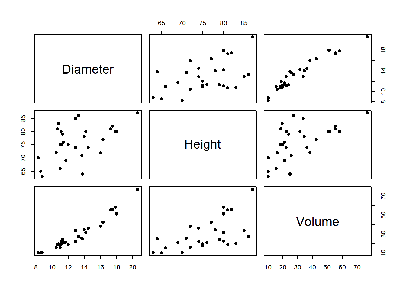
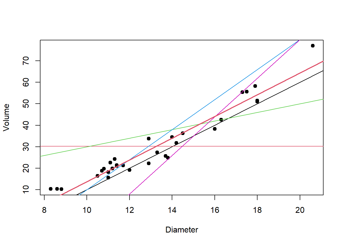
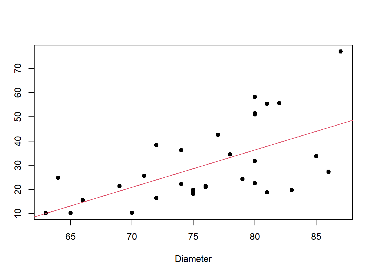
#### Regression line:

# We can consider several lines passing through the scatterplot:
plot(trees$Diameter, trees$Volume, pch=19,
     ylab="Volume", xlab = "Diameter")
abline(a=-40, b=5, col=1)
abline(h=mean(trees$Volume), col=2)
abline(a=10, b=2, col=3)
abline(a=-60, b=7, col=4)
abline(a=-100, b=9, col=6)


# Let's estimate the regression line,
# that is the BEST line passing through the data:
lm1 <- lm(Volume ~ Diameter, data=trees)
summ1 <- summary(lm1);summ1

Call:
lm(formula = Volume ~ Diameter, data = trees)

Residuals:
   Min     1Q Median     3Q    Max 
-8.065 -3.107  0.152  3.495  9.587 

Coefficients:
            Estimate Std. Error t value Pr(>|t|)    
(Intercept) -36.9435     3.3651  -10.98 7.62e-12 ***
Diameter      5.0659     0.2474   20.48  < 2e-16 ***
---
Signif. codes:  0 '***' 0.001 '**' 0.01 '*' 0.05 '.' 0.1 ' ' 1

Residual standard error: 4.252 on 29 degrees of freedom
Multiple R-squared:  0.9353,    Adjusted R-squared:  0.9331 
F-statistic: 419.4 on 1 and 29 DF,  p-value: < 2.2e-16

abline(lm1, col=2,lwd=2)

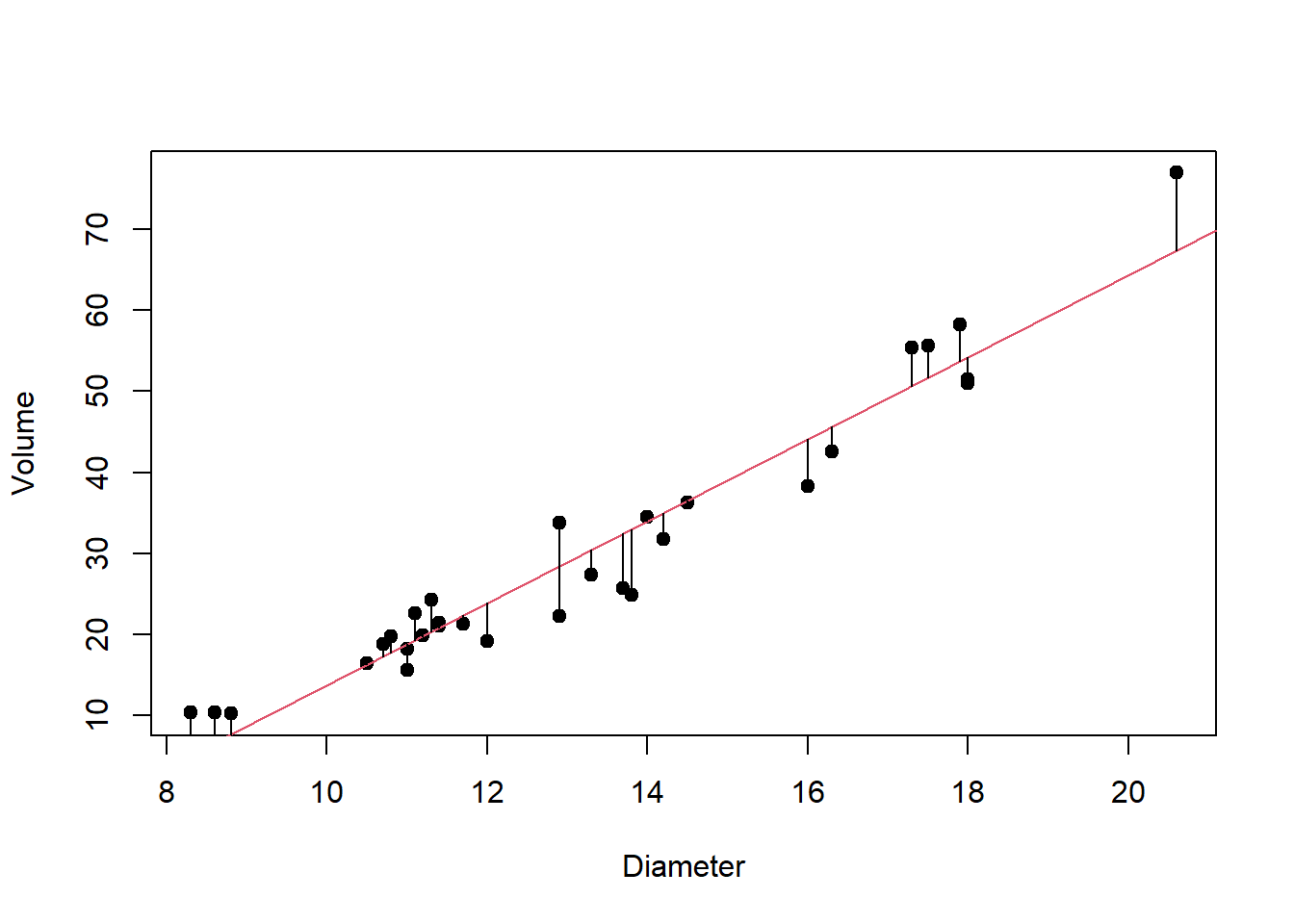
# Let's look at the regression line:
plot(trees$Diameter, trees$Volume, pch=19,
     ylab="Volume", xlab = "Diameter")
abline(lm1, col=2)


# Compute the predicted values of the model:
coef(lm1)[1] + coef(lm1)[2]*trees$Diameter

 [1]  5.103149  6.622906  7.636077 16.248033 17.261205 17.767790 18.780962
 [8] 18.780962 19.287547 19.794133 20.300718 20.807304 20.807304 22.327061
[15] 23.846818 28.406089 28.406089 30.432431 32.458774 32.965360 33.978531
[22] 34.991702 36.511459 44.110244 45.630001 50.695857 51.709028 53.735371
[29] 54.241956 54.241956 67.413183

y_prev <- predict(lm1)

y_prev == coef(lm1)[1] + coef(lm1)[2]*trees$Diameter

   1    2    3    4    5    6    7    8    9   10   11   12   13   14   15   16 
TRUE TRUE TRUE TRUE TRUE TRUE TRUE TRUE TRUE TRUE TRUE TRUE TRUE TRUE TRUE TRUE 
  17   18   19   20   21   22   23   24   25   26   27   28   29   30   31 
TRUE TRUE TRUE TRUE TRUE TRUE TRUE TRUE TRUE TRUE TRUE TRUE TRUE TRUE TRUE 

#### Residuals:
# Once we fitted the model, we can compute the residuals
e <- trees$Volume - y_prev

# Graphical representation of the residuals:
segments(x0=trees$Diameter, x1=trees$Diameter,
         y0=trees$Volume, y1=y_prev)

# Estimate of sigma^2
SSres <- sum(e^2)
sigma2_hat <- SSres/(n-2)
sqrt(sigma2_hat)

[1] 4.251988

SStot <- var(trees$Volume)*(n-1)
SSreg <- sum((y_prev - mean(trees$Volume))^2)

SSreg # spiegata

[1] 7581.781

SSres # residua

[1] 524.3025

SStot # totale

[1] 8106.084

# Deviance decomposition:
round(SStot, 8) == round(SSres + SSreg, 8) 

[1] TRUE

# R^2:
R2 <- SSreg/SStot; R2

[1] 0.9353199

(cor(trees$Diameter, trees$Volume))^2

[1] 0.9353199

# Design matrix:
X <- cbind(1, trees$Diameter); X

      [,1] [,2]
 [1,]    1  8.3
 [2,]    1  8.6
 [3,]    1  8.8
 [4,]    1 10.5
 [5,]    1 10.7
 [6,]    1 10.8
 [7,]    1 11.0
 [8,]    1 11.0
 [9,]    1 11.1
[10,]    1 11.2
[11,]    1 11.3
[12,]    1 11.4
[13,]    1 11.4
[14,]    1 11.7
[15,]    1 12.0
[16,]    1 12.9
[17,]    1 12.9
[18,]    1 13.3
[19,]    1 13.7
[20,]    1 13.8
[21,]    1 14.0
[22,]    1 14.2
[23,]    1 14.5
[24,]    1 16.0
[25,]    1 16.3
[26,]    1 17.3
[27,]    1 17.5
[28,]    1 17.9
[29,]    1 18.0
[30,]    1 18.0
[31,]    1 20.6

solve((t(X)%*%X))

            [,1]         [,2]
[1,]  0.62635938 -0.044843294
[2,] -0.04484329  0.003384812

# The summary contains several information:
names(summ1)

 [1] "call"          "terms"         "residuals"     "coefficients" 
 [5] "aliased"       "sigma"         "df"            "r.squared"    
 [9] "adj.r.squared" "fstatistic"    "cov.unscaled" 

summ1$cov.unscaled

            (Intercept)     Diameter
(Intercept)  0.62635938 -0.044843294
Diameter    -0.04484329  0.003384812

summ1$residuals

         1          2          3          4          5          6          7 
 5.1968508  3.6770939  2.5639226  0.1519667  1.5387954  1.9322098 -3.1809615 
         8          9         10         11         12         13         14 
-0.5809615  3.3124528  0.1058672  3.8992815  0.1926959  0.5926959 -1.0270610 
        15         16         17         18         19         20         21 
-4.7468179 -6.2060887  5.3939113 -3.0324313 -6.7587739 -8.0653595  0.5214692 
        22         23         24         25         26         27         28 
-3.2917021 -0.2114590 -5.8102436 -3.0300006  4.7041430  3.9909717  4.5646292 
        29         30         31 
-2.7419565 -3.2419565  9.5868168 

###################################
#### Regression plane:

# We consider an additional covariate:
lm2 <- lm(Volume ~ Diameter + Height, data=trees)
summ2 <- summary(lm2); summ2

Call:
lm(formula = Volume ~ Diameter + Height, data = trees)

Residuals:
    Min      1Q  Median      3Q     Max 
-6.4065 -2.6493 -0.2876  2.2003  8.4847 

Coefficients:
            Estimate Std. Error t value Pr(>|t|)    
(Intercept) -57.9877     8.6382  -6.713 2.75e-07 ***
Diameter      4.7082     0.2643  17.816  < 2e-16 ***
Height        0.3393     0.1302   2.607   0.0145 *  
---
Signif. codes:  0 '***' 0.001 '**' 0.01 '*' 0.05 '.' 0.1 ' ' 1

Residual standard error: 3.882 on 28 degrees of freedom
Multiple R-squared:  0.948, Adjusted R-squared:  0.9442 
F-statistic:   255 on 2 and 28 DF,  p-value: < 2.2e-16

library(scatterplot3d)
library(plotly)

Caricamento del pacchetto richiesto: ggplot2

Caricamento pacchetto: 'plotly'

Il seguente oggetto è mascherato da 'package:ggplot2':

    last_plot

Il seguente oggetto è mascherato da 'package:stats':

    filter

Il seguente oggetto è mascherato da 'package:graphics':

    layout

plot3d <- scatterplot3d(trees$Diameter, trees$Height, trees$Volume, 
        angle=40, scale.y=0.7, pch=16, color ="red", 
       # angle=40, scale.y=0.7, pch=16, color ="red", 
        main ="Regression Plane")
plot3d$plane3d(lm2, lty.box = "solid")
plot3d$points3d(trees$Diameter, trees$Height, trees$Volume,col="blue", type="h", pch=16)

step(lm2)

Start:  AIC=86.94
Volume ~ Diameter + Height

           Df Sum of Sq    RSS     AIC
<none>                   421.9  86.936
- Height    1     102.4  524.3  91.671
- Diameter  1    4783.0 5204.9 162.824

Call:
lm(formula = Volume ~ Diameter + Height, data = trees)

Coefficients:
(Intercept)     Diameter       Height  
   -57.9877       4.7082       0.3393  

##################################
#### Dummy:

trees$Height_factor <- factor(ifelse(trees$Height < 76, "Basso", "Alto"))
str(trees)

'data.frame':   31 obs. of  4 variables:
 $ Diameter     : num  8.3 8.6 8.8 10.5 10.7 10.8 11 11 11.1 11.2 ...
 $ Height       : num  70 65 63 72 81 83 66 75 80 75 ...
 $ Volume       : num  10.3 10.3 10.2 16.4 18.8 19.7 15.6 18.2 22.6 19.9 ...
 $ Height_factor: Factor w/ 2 levels "Alto","Basso": 2 2 2 2 1 1 2 2 1 2 ...

lm_dummy <- lm(Volume ~ Diameter + Height_factor, data=trees)
summary(lm_dummy)

Call:
lm(formula = Volume ~ Diameter + Height_factor, data = trees)

Residuals:
    Min      1Q  Median      3Q     Max 
-5.6703 -3.0292 -0.6302  2.9008  9.9239 

Coefficients:
                   Estimate Std. Error t value Pr(>|t|)    
(Intercept)        -31.1856     3.7955  -8.216 6.08e-09 ***
Diameter             4.7700     0.2534  18.827  < 2e-16 ***
Height_factorBasso  -4.0699     1.5716  -2.590   0.0151 *  
---
Signif. codes:  0 '***' 0.001 '**' 0.01 '*' 0.05 '.' 0.1 ' ' 1

Residual standard error: 3.887 on 28 degrees of freedom
Multiple R-squared:  0.9478,    Adjusted R-squared:  0.9441 
F-statistic: 254.3 on 2 and 28 DF,  p-value: < 2.2e-16

plot(Volume ~ Diameter, data=trees, col=Height_factor, pch=20)
abline(a=-31.1856, b=4.7700, col=1)
abline(a=-31.1856-4.0699, b=4.7700, col=2)
legend(8,70, legend=c("Alto","Basso"), col=1:2, lty=1, bty = "n")

##################################
#### Polynomial regression:
cor(trees[,1:3])

          Diameter    Height    Volume
Diameter 1.0000000 0.5192801 0.9671194
Height   0.5192801 1.0000000 0.5982497
Volume   0.9671194 0.5982497 1.0000000

plot(trees$Height, trees$Volume, pch=19,
     ylab="Volume", xlab = "Diameter")
lm_poly_1 <- lm(Volume ~ Height, data=trees)
summary(lm_poly_1)

Call:
lm(formula = Volume ~ Height, data = trees)

Residuals:
    Min      1Q  Median      3Q     Max 
-21.274  -9.894  -2.894  12.068  29.852 

Coefficients:
            Estimate Std. Error t value Pr(>|t|)    
(Intercept) -87.1236    29.2731  -2.976 0.005835 ** 
Height        1.5433     0.3839   4.021 0.000378 ***
---
Signif. codes:  0 '***' 0.001 '**' 0.01 '*' 0.05 '.' 0.1 ' ' 1

Residual standard error: 13.4 on 29 degrees of freedom
Multiple R-squared:  0.3579,    Adjusted R-squared:  0.3358 
F-statistic: 16.16 on 1 and 29 DF,  p-value: 0.0003784

abline(lm_poly_1, col=2)

lm_poly_2 <- lm(Volume ~ Height + I(Height^2), data=trees)
summ_poly_2 <- summary(lm_poly_2)
lm_poly_3 <- lm(Volume ~ Height + I(Height^2) + I(Height^3), data=trees)
summ_poly_3 <- summary(lm_poly_3)

quad <- function(h, model){
  coef <- coef(model)
  x <- coef[1] + coef[2]*h + coef[3]*h^2
  return(x)
}

cubic <- function(h, model){
  coef <- coef(model)
  x <- coef[1] + coef[2]*h + coef[3]*h^2 + coef[4]*h^3
  return(x)
}

plot(trees$Height, trees$Volume, pch=19,
     ylab="Volume", xlab = "Diameter")
abline(lm_poly_1, col=2)
curve(quad(x, lm_poly_2), add=T, col=3)
curve(cubic(x, lm_poly_3), add=T, col=4)

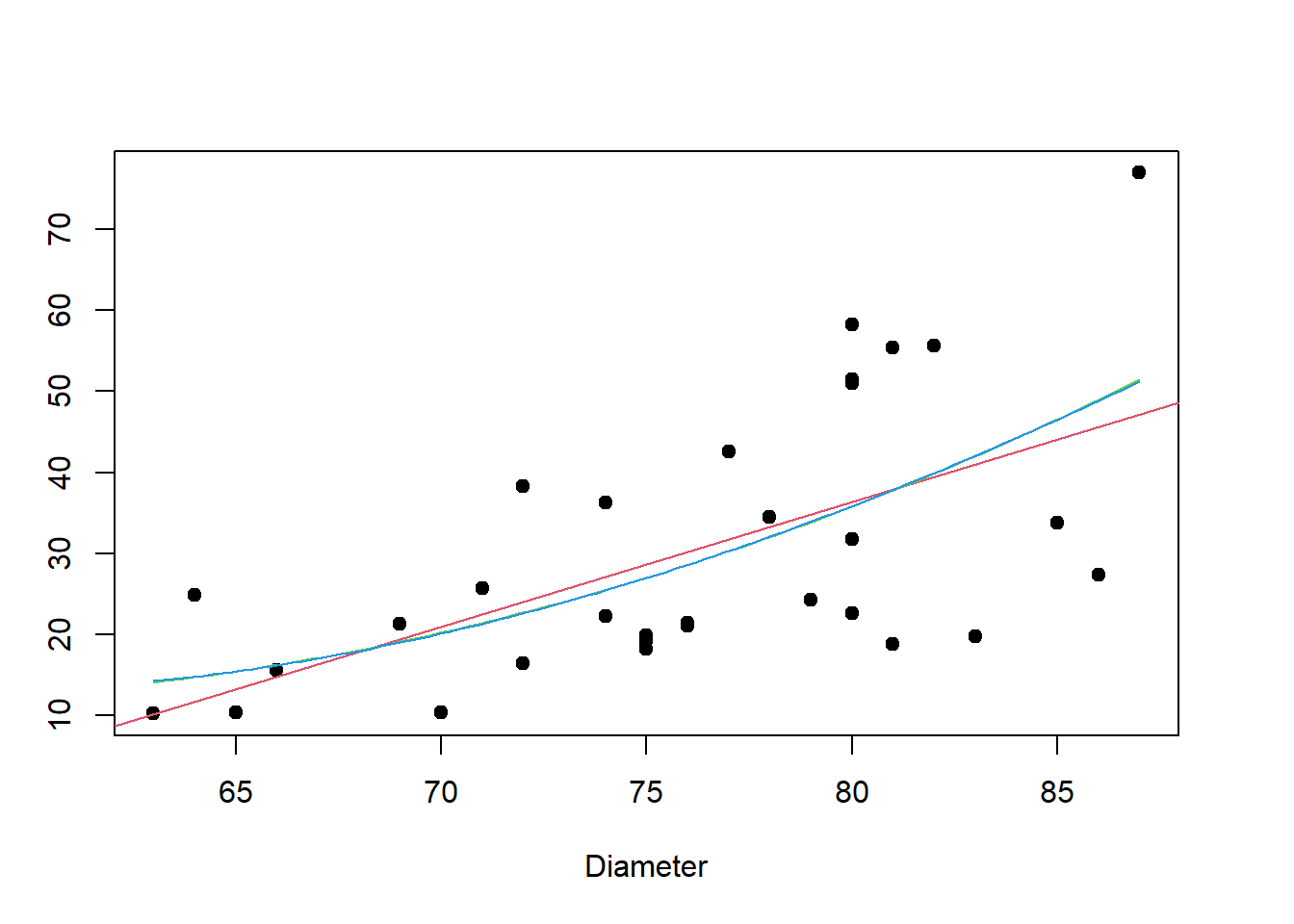
# The anova function compares two models:
# If we accept the hypothesis that the two models 
# have the same fit, then we prefer the simpler one
anova(lm_poly_1, lm_poly_3)

Analysis of Variance Table

Model 1: Volume ~ Height
Model 2: Volume ~ Height + I(Height^2) + I(Height^3)
  Res.Df    RSS Df Sum of Sq      F Pr(>F)
1     29 5204.9                           
2     27 5106.1  2    98.815 0.2613  0.772

##################################

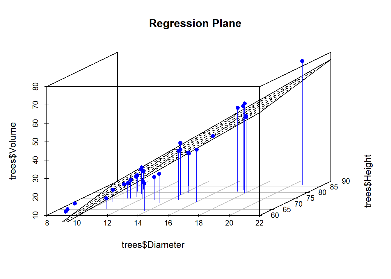
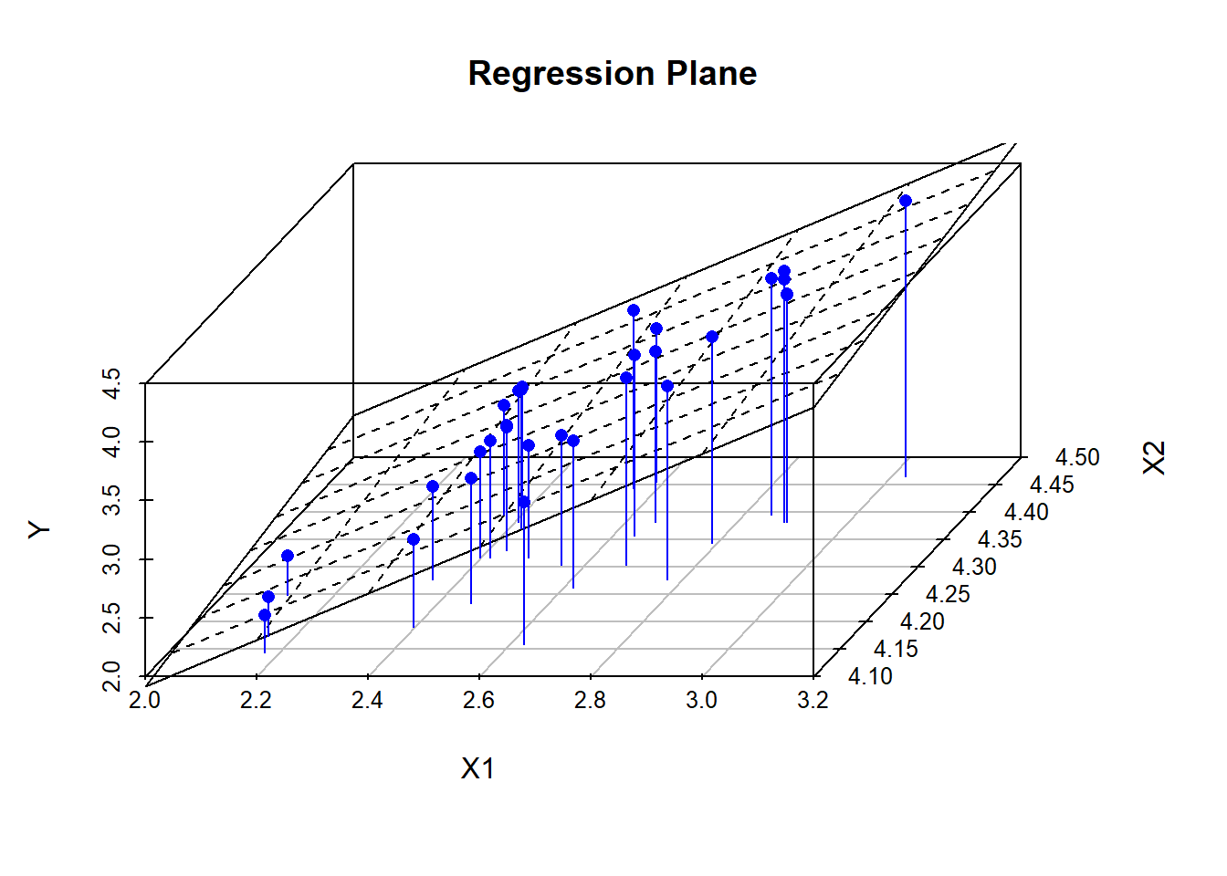
# Let us suppose that a tree is a cylinder.
# We know that the volume of a cylinder
# is V = pi * (Diameter/2)^2 * Height

# Then log(V) = log(pi/4) + 2log(Diameter) + log(Height)
Y <- log(trees$Volume)
X1 <- log(trees$Diameter)
X2 <- log(trees$Height)

lm_log <- lm(Y ~ X1 + X2)
summary(lm_log)

Call:
lm(formula = Y ~ X1 + X2)

Residuals:
      Min        1Q    Median        3Q       Max 
-0.168561 -0.048488  0.002431  0.063637  0.129223 

Coefficients:
            Estimate Std. Error t value Pr(>|t|)    
(Intercept) -6.63162    0.79979  -8.292 5.06e-09 ***
X1           1.98265    0.07501  26.432  < 2e-16 ***
X2           1.11712    0.20444   5.464 7.81e-06 ***
---
Signif. codes:  0 '***' 0.001 '**' 0.01 '*' 0.05 '.' 0.1 ' ' 1

Residual standard error: 0.08139 on 28 degrees of freedom
Multiple R-squared:  0.9777,    Adjusted R-squared:  0.9761 
F-statistic: 613.2 on 2 and 28 DF,  p-value: < 2.2e-16

plot3d <- scatterplot3d(X1, X2, Y, 
                        angle=60, scale.y=0.7, pch=16, color ="red", 
                        main ="Regression Plane")
plot3d$plane3d(lm_log, lty.box = "solid")
plot3d$points3d(X1, X2, Y,col="blue", type="h", pch=16)